Nyquist Plot: Understanding Frequency Response & Stability
If you’re traversing the world of control systems, you’ll likely encounter the Nyquist plot—a vital tool for analyzing system stability. This graphical representation helps you assess how a system responds to different frequencies, offering insights into potential instabilities. By examining how the plot encircles the critical point, you can gauge the presence of unstable poles and zeros. But how does this translate to real-world applications? There’s much more to uncover.
Key Takeaways
- Nyquist plots visualize the frequency response of a system’s open-loop transfer function in the complex plane.
- They help assess system stability through encirclements around the critical point (-1, 0).
- Encirclement patterns in Nyquist plots indicate unstable poles and zeros influencing system stability.
- Time delays in systems introduce phase shifts, complicating Nyquist plot analysis and stability evaluation.
- Tools like MATLAB and Simulink facilitate Nyquist plot creation and analysis for control system behavior.
Overview of Nyquist Stability Criterion
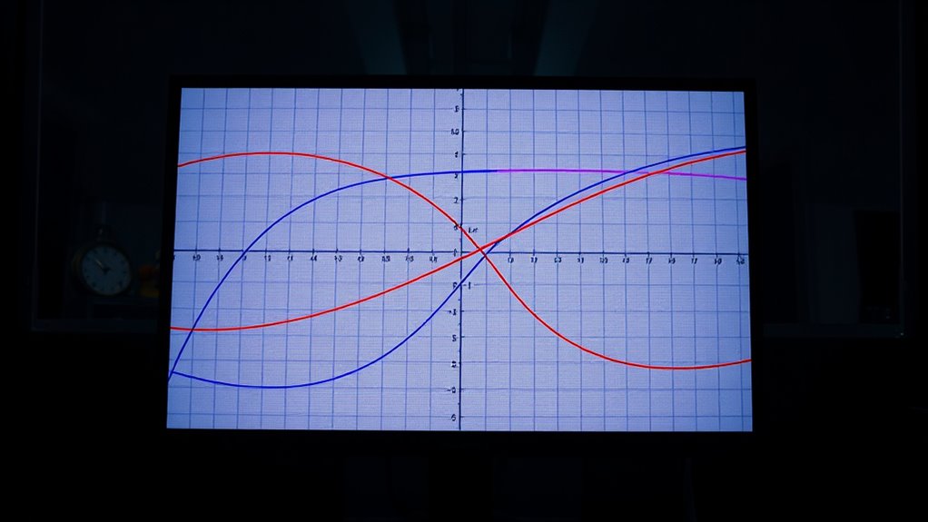
When analyzing the stability of linear dynamical systems, the Nyquist Stability Criterion offers a robust graphical method by focusing on the frequency response of the open-loop transfer function.
You’ll use a Nyquist plot to visualize this response, with the real part on the x-axis and the imaginary part on the y-axis. The key to evaluating stability is observing how the plot encircles the point (-1, 0). These encirclements help determine the stability margins of your system.
To predict the behavior of the closed-loop transfer function, count the counterclockwise encirclements and apply the formula Z = N + P. This approach is particularly useful in control engineering, as it accommodates systems with delays and non-rational transfer functions without explicitly computing poles and zeros.
Characteristics of Nyquist Plots
When examining Nyquist Plots, you’ll notice they provide a powerful visual tool for evaluating system stability through encirclements of the point (-1, 0).
The plot’s depiction of frequency response, with real and imaginary components, helps you identify critical stability indicators such as right half-plane poles and zeros.
However, be cautious of time delays in your system, as they introduce complexities like increased negative phase shifts that complicate your stability analysis.
Encirclement and Stability Indicators
Although analyzing a control system’s stability might seem complex, the Nyquist plot offers an intuitive way to assess it by focusing on the encirclement of the point (-1, 0).
You can use the Nyquist stability criterion to determine a closed-loop system‘s stability. The plot’s encirclement pattern reveals the number of unstable poles and zeros. If the plot encircles the -1 point counterclockwise, it indicates an unstable pole. Conversely, clockwise encirclements suggest right half-plane zeros.
Count the net encirclements (N) and add them to the right half-plane poles (P) to calculate closed-loop zeros (Z) using Z = N + P.
Frequency Response Representation
As you explore the characteristics of Nyquist plots, you’ll discover they offer a powerful visualization of a system’s frequency response. These plots map the real and imaginary parts of a transfer function, illustrating how gain and phase change across frequencies, which is critical for stability analysis. By observing encirclements around the crucial point (-1, 0), you can assess the system’s stability. The logarithmic frequency sweep enhances your understanding, highlighting critical frequencies for determining stability margins. Nyquist plots reveal complex behaviors through poles and zeros, guiding you to insights about gain and phase margins.
Here’s a summary table:
| Aspect | Role in Nyquist Plots | Importance |
|---|---|---|
| Real vs. Imaginary | Maps frequency response | Visualizes system behavior |
| Stability Analysis | Assesses encirclements | Determines stability margins |
| Log Frequency Sweep | Highlights critical frequencies | Enhances system understanding |
Impact of System Delays
Understanding the role of Nyquist plots in frequency response representation sets the stage for exploring how system delays impact these visualizations.
Time delays introduce negative phase shifts that reshape the Nyquist plot, affecting its stability characteristics. As the delay grows, the plot may spiral toward the origin, complicating stability analysis by causing encirclements of the -1+j0 point. This can push a stable system into instability, even if there are no unstable poles initially.
You’ll need to evaluate the phase and gain margins carefully, as these delays might push poles in the right direction, exceeding stability thresholds. Traditional methods relying on characteristic equation roots won’t suffice because delays add complexities that aren’t captured in polynomial analysis, challenging your stability assessments.
Mathematical Foundations of the Nyquist Criterion
The Nyquist Criterion offers a powerful tool for evaluating system stability by leveraging the Laplace transform to connect a system’s frequency response to its stability characteristics.
You start with the open-loop transfer function, G(s), from which you derive the characteristic equation. This equation plays an essential role in determining stability by indicating how many times the Nyquist plot encircles the point (-1, 0).
The relationship Z = N + P links the number of right half plane (RHP) zeros (Z) with the number of encirclements (N) and the number of RHP poles (P).
Stability Analysis Using Nyquist Plots

When analyzing stability using Nyquist plots, pay attention to how many times the plot encircles the critical point (-1, 0), as this indicates stability or potential instability.
Time delays in your system can cause additional phase shifts, leading to more encirclements of the -1 point and complicating your stability assessment.
Encirclement and Stability Indicators
Although analyzing system stability might seem complex, the Nyquist plot offers a clear method for determining it through encirclement of the critical point (-1, 0). By examining counterclockwise encirclements, you can assess potential instability, particularly when right half-plane (RHP) poles are present in the open-loop transfer function.
The Nyquist Stability Criterion states that for each RHP pole, the plot must encircle -1 counterclockwise to guarantee closed-loop stability. A system is stable if there are no encirclements of the -1 point. However, a clockwise encirclement indicates instability, especially if the open-loop system has RHP poles.
The balance between clockwise and counterclockwise encirclements directly impacts stability, calculated using Z = N + P, where N is counterclockwise encirclements, and P is RHP poles.
Impact of Time Delays
Understanding system stability through the Nyquist plot involves examining encirclements of the critical point (-1, 0). When time delays are present, they introduce additional phase lag, which can greatly distort the Nyquist plot.
This distortion often spirals the plot closer to the origin, raising stability issues by increasing the likelihood of encircling the critical point. As these delays grow, the phase shift becomes even more negative, complicating your stability analysis.
You might notice complex behaviors like additional encirclements, indicating a potential shift from stability to instability. Since time delays affect system dynamics, you can’t rely solely on the characteristic equation roots.
Instead, analyze the Nyquist plot for encirclements and phase shifts. Simulation tools can help visualize these impacts and assess stability margins.
Impact of Time Delays on Nyquist Plots
As you explore the impact of time delays on Nyquist plots, you’ll notice that these delays introduce additional negative phase shifts, greatly affecting system stability.
Time delays can push the phase closer to the critical -180 ° point, considerably altering stability characteristics. As the delay increases, the Nyquist plot may spiral towards the origin, complicating analysis and potentially leading to encirclements of the -1 point, which indicates instability.
These delays can cause the plot to exhibit complex behaviors, including multiple loops and oscillations, making visual stability assessments challenging.
Stability margins, such as gain and phase margins, are particularly sensitive to time delays, as even small delays can drastically reduce them. Therefore, a careful assessment is essential, as traditional methods may overlook these effects.
Example Cases of Nyquist Plots
Having explored how time delays impact Nyquist plots and affect system stability, let’s now look at specific example cases to illustrate these concepts in action.
In the simplest scenario, a Nyquist plot with no encirclement of the -1+j0 point signifies system stability, with no right half-plane poles. When a pole exists at the origin, the plot detours around it, showing stability and a gain margin of 3.52 dB.
If a right half-plane pole is present, an encirclement of the -1+j0 point counterclockwise indicates stability despite the pole. Conversely, a clockwise encirclement with a right half-plane pole suggests instability.
Finally, a double pole at the origin introduces complex plot behavior, but still confirms stability without encirclement.
Simulation Tools for Nyquist Stability Analysis
When it comes to analyzing system stability using Nyquist plots, simulation tools like MATLAB and Simulink are invaluable. They enable you to visualize control system behavior and stability margins, thereby bridging theory and practice. MATLAB’s specialized functions for Nyquist plots simplify analyzing open-loop and closed-loop stability without manual calculations. Simulink offers real-time feedback, showing how parameter variations, like time delays, affect system stability.
For impedance spectrum analysis, the EIS Spectrum Analyser freeware is also a great choice, letting you visualize Nyquist plots from experimental data. These tools enhance your understanding of control system dynamics and stability.
| Tool | Functionality | Benefit |
|---|---|---|
| MATLAB | Nyquist plot generation | Simplifies stability analysis |
| Simulink | Real-time simulation | Visualizes dynamic behavior |
| EIS Spectrum Analyser | Impedance spectrum analysis | Visualizes experimental data |
Comparing Nyquist and Bode Plots
While analyzing control systems, you’ll encounter both Nyquist and Bode plots, each offering unique insights.
Nyquist plots excel in revealing system stability by highlighting frequency response and encirclements of the -1 point. They accurately handle right half-plane poles, providing a definitive stability analysis through encirclement techniques.
In contrast, Bode plots focus on magnitude and phase across frequencies, which might miss stability issues in systems with these poles.
Nyquist plots can directly show the number of right-half-plane zeros and poles, unlike Bode plots. They’re particularly effective for systems with time delays, visualizing negative phase effects on stability.
Historical Context and Resources
Understanding the unique insights offered by Nyquist plots leads us naturally to investigate their historical roots and available resources. Introduced by Harry Nyquist in 1932, this plot focuses on system stability through frequency response analysis, which is essential in understanding the Nyquist Stability Criterion.
As you explore linear control theory, recognize the contributions of scholars like Reinschke and Strecker, who expanded on its significance. Nyquist plots help analyze transfer functions, especially those with right half-plane poles and zeros, which are vital for determining stability.
For hands-on exploration, educational resources like Mathematics LibreTexts and MATLAB provide tools to craft and interpret these plots. Additionally, archived materials on Wikimedia Commons support visual learning and deepen your grasp of system stability.
Conclusion
In your exploration of Nyquist plots, you’ve discovered a powerful tool for evaluating control system stability. By analyzing these plots, you can gauge the presence of unstable poles and zeros, guiding essential design decisions. Nyquist plots, with their unique ability to depict frequency response, offer insights that complement other methods like Bode plots. As you apply these concepts, remember the impact of time delays and leverage simulation tools to enhance your understanding and system design.
FAQs
1. How to Interpret the Nyquist Plot?
You evaluate system stability by checking encirclements of the critical point. Count counterclockwise encirclements to assess instability. If the plot doesn’t circle the point, the system is stable. Adjust gain and phase for desired stability margins.
2. How to Check Stability Using Nyquist Plot?
To check stability, count the counterclockwise encirclements of the point (-1, 0). Zero encirclements mean stability if there are no RHP poles. If RHP poles exist, each requires one encirclement for stability.
3. What Is a Nyquist and Bode Plot?
You’re asking about Nyquist and Bode plots. Nyquist plots graphically show system stability by plotting real and imaginary parts, while Bode plots display gain and phase over frequency. Together, they help you analyze and understand system dynamics effectively.
4. What Are the Advantages and Disadvantages of the Nyquist Plot?
You’re analyzing system stability. You’ve got a tool that visually assesses phase and gain margins, even for complex systems. However, it struggles with complexity and imaginary axis poles, which can lead to inaccuracies if conditions aren’t met.